

The purpose of this project is to implement some machine learning algorithms to try and predict whether a team will run or pass on second down, using the 2015 NFL Play-By-Play dataset. Here is a link to the relevant jupyter notebook.
Before applying any sophisticated techniques, we consider a couple of basic prediction strategies. One such strategy is to simply always choose pass, since teams choose to pass on second down 58% of the time. On the other hand, if it is second and short, teams tend to run more than pass, as the following graphic shows.
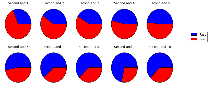
This suggests that we can get a decent prediction by choosing run when it is second down with five yards or fewer to go, and pass otherwise. Indeed, this results in a 62.6% accuracy when tested against our dataset. Our goal is to try to beat these simple predictions using machine learning techniques.
First we must prepare our data. It is convenient to limit ourselves to two features for our predictions. By doing this, we may easily visualize our results by plotting them in the xy-plane. We use the sklearn method SelectKBest to choose the best two features from our dataset.

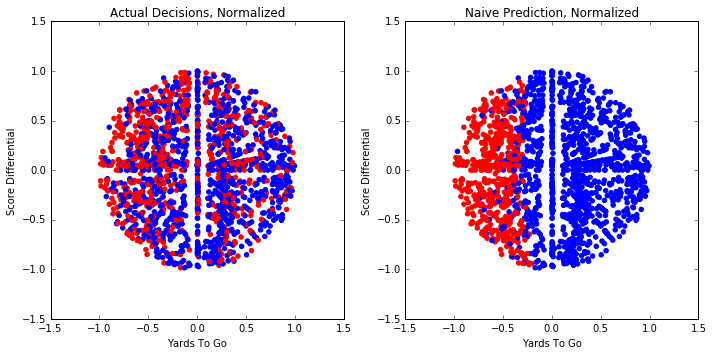
Based on these results, we choose the number of yards to go for a first down, as well as score differential, as the two features we will be using for our predictions. Next we separate our data into two subsets. Namely, we have a training subset consisting of 80% of the data, and a testing subset consisting of the other 20%. Here is a plot of the testing data, with run in red and pass in blue. The first plot represents the actual play calls and the second is our naive prediction.

Some of the algorithms we will be using work better with our features normalized and standardized. Normalizing will scale the features so they take values between 0 and 1. Standardizing gives the data a standard normal distribution. Here is a plot of the same data we just showed, with the features normalized and standardized.
Now we can start playing with some machine learning algorithms! We’ll start with logistic regression. With sklearn it is as simple as running the following code:
logistic = LogisticRegression()
logistic.fit(X_train, y_train)

logistic_prediction = logistic.predict(X_test)
We write a function graphPredict to graph the prediction and give the accuracy. Plugging in our logistic regression model results in the following graph:
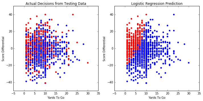
This results in a 63.6% accuracy on our testing set. We also run the cross_val_score function to find the accuracy on 5 different test/training splits, which when averaged together still results in a 63.6% accuracy. So the prediction obtained by logistic regression seems to be slightly better than the naive prediction.
We run the same procedure using other common classification algorithms, including: k-Nearest Neighbors, Support Vector Machines, Decision Trees, and Random Forests. Here are the resulting graphs and accuracies of these algorithms.
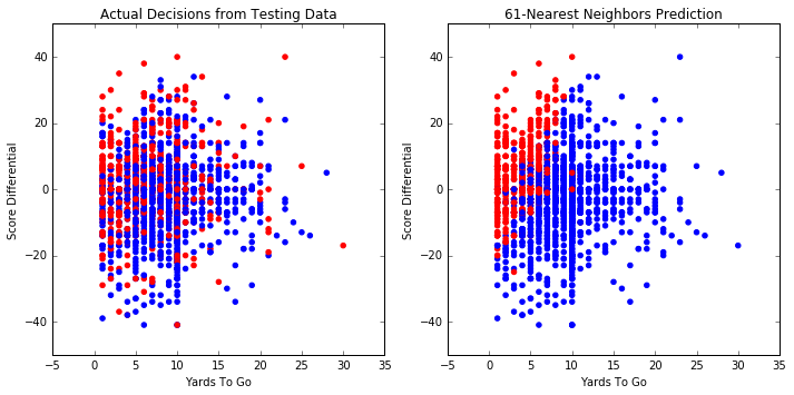
Accuracy on testing set: 64.8%
Average score on 5 splits: 64.9%
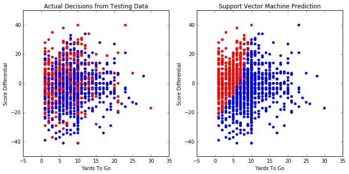
Accuracy on testing set: 63.9%
Average score on 5 splits: 64.0%
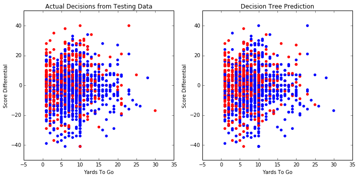
Accuracy on testing set: 56.1%
Average score on 5 splits: 57.5%
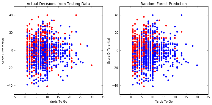
Accuracy on testing set: 61.6%
Average score on 5 splits: 62.5%
In conclusion, a few of these algorithms give us slightly better results than the naive strategy. They can probably be improved by using more features, and by choosing our parameters more carefully. For instance, how many neighbors would give the best result for k-NN? How many estimators should we use for random forests? Should we use a linear or polynomial (and what degree?) kernel for our support vector machine? We will tackle these issues in another post. Our new goal is to come up with a strategy which predicts correctly at least 70% of the time.